8. Quick Labeling

The EO Time Series Viewer assists you in describing, i.e. label reference data. Whether your locations (vector point, lines or polygons) already exist, or need to be digitized on a visualized maps, in both cases you want to describe them with individual attributes. Such attributes can be of different type. For example land cover labels (landcover=’pasture’) time stamps that indicate a change event (deforestation=’2024-04-03’), or numeric values (soil_fraction=0.3).

The EO Time Series Viewer supports this with “Quick Label” short-cuts. If triggered, they send fill values into one or multuple attribute cells of selected vector features. Such features could be the points or polygons of a vector layer, that have been selected in a map, an attribute table, or a temporal profile plot temporal profile plot.

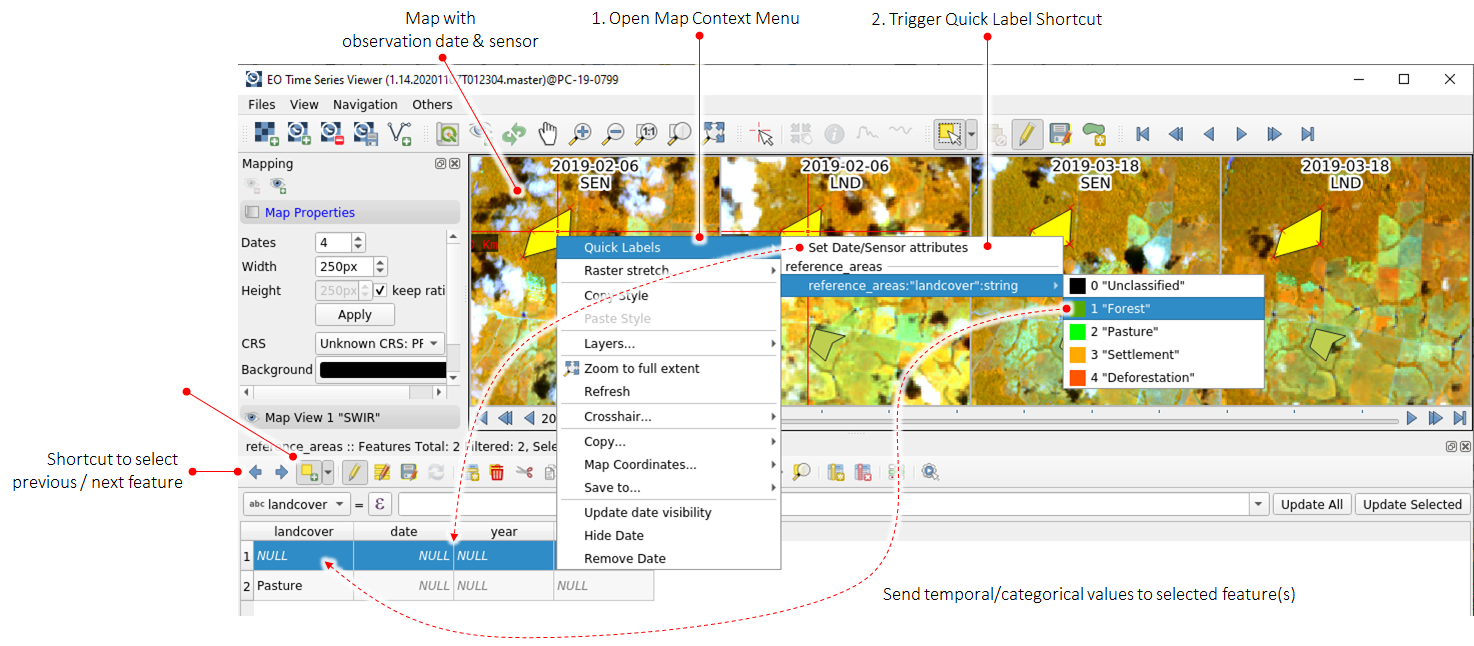
Fig. 8.1 Quick labeling workflow, triggered from a map canvas contex menu

8.1. Shortcuts

The following table shows the quick label types that you can setup to fill in attribute values.

Type	Supported Field Types	Description
Off	Any	Does nothing. Useful to pause quick labeling
Date	String, Date	Date taken from the map canvas or cursor position of time series plot
DateTime	String, DateTime	Date-Time stamp taken from the map canvas date or cursor position of time series plot
Time	String, Time	Time stamp taken from the map canvas date or cursor position of time series plot
DOY	String, Integer	Day of year taken from the map canvas date or cursor position of time series plot
Year	String, Integer	Year taken from the map canvas date or cursor position of time series plot
DecimalYear	String, Float	Decimal year value taken from the map canvas date or cursor position of time series plot
Sensor	String	Name of sensor (as defined in the sensor panel) relating to the observation that is shown in the map canvas
SourceImage	String	Path of raster observation that is shown below the mouse cursor
Customized	String	Value returned from the evaluation of a user defined expression.
Classification	String, Integer	Class name or label number, selectable from context menu

8.2. Example

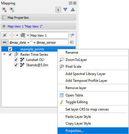
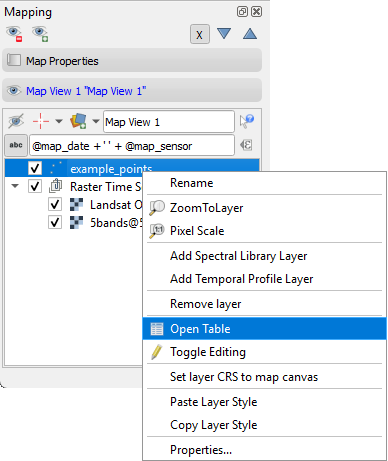
Start the EO Time Series Viewer and open the example data (Files > Add example). The layer tree contains now an example_points layer. Use the context menu to open its layer properties.

The example_points.geojson has five fields of different data types. We like to use them to store the following values:

Field	Expected Values
landcover	A landcover label like forest, deforestation, water, burnt area or pasture
date	The observation date on which we observed the landcover.
doy	The day-of-year of the observation date, as integer number.
Image	The path of the raster image in which we observed the landcover.

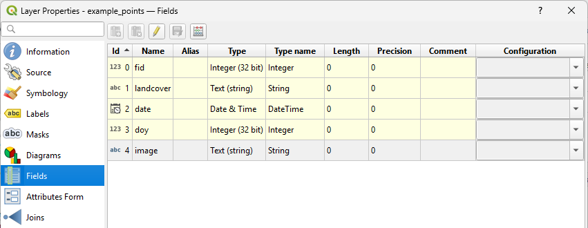
Fig. 8.2.1 Layer properties with Fields page

The Attribute Form is used to setup the Quick Labeling short-cuts. Select the landcover field, set the Widget Type combobox to EOTSV Quick Label and then the Type combobox to Classification. The classification widgets allows you to define a classification scheme. Each class has a numeric label, a name and a color.

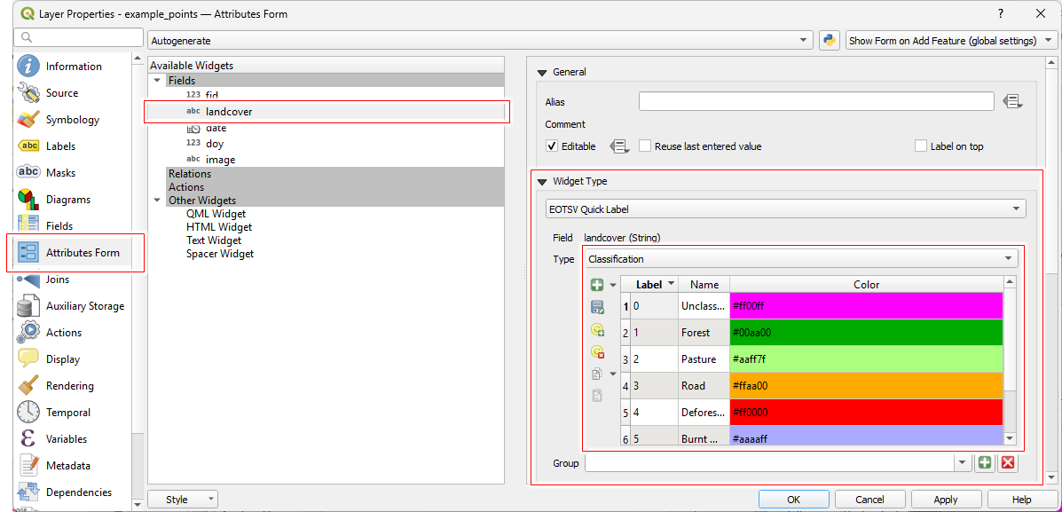
Fig. 8.2.2 Layer property Attributes Form with quick label classification activated for the classification field.

Now set the other fields to the following quick label types:

Field	Widget Type	Quick Label Type
landcover	EOTSV Quick Label	Classification
date	EOTSV Quick Label	DateType
doy	EOTSV Quick Label	DOY
image	EOTSV Quick Label	SourceImage

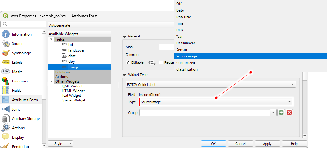
Fig. 8.2.3 Layer property Attributes Form, having the quick label source image path activated for the image field.

When done, Apply the changes and click Ok to close the layer settings. Now we are ready to use quick labeling shortcuts. To see how they fill in attribute values, open the attribute table of the example_points layer.

From now on, the map context menu offers quick label shortcuts. If triggered, they write the derived date or time data, or the selected class information into the attributes of selected vector features. This ca save you a lot of time, as these attributes no longer have to be entered individually, and are also written for multiple selected features at once.

Using the and buttons selects the next (or previous) vector feature and pans the maps too.

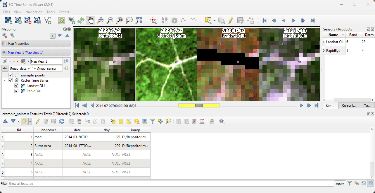
Fig. 8.2.4 Quick labels are set from the map context menu. Attributes are derived from the map observation date or map layers and written into the attributes of selected vector features.

Todo

Add example with quick label context menu for temporal profile plot.

8.3. Label Groups

In some cases it can be helpful to use a label shortcut type to fill different attributes with different values. For example, do describe the progress of land clearing in tropical landscapes similar to Jakimow et al. 2023, we want to use short cuts to collect the Date and SourceImage for the following successive steps:

Table 8.3.1 Land clearing steps and related vector attributes to fill with quick label shortcuts

Management	Attribute	Description
deforestation	def_date	date where deforestation becomes visible the 1st time
	def_img	path of image related to def_date
burning	bur_date	date of burning of slashed vegetation
	bur_img	path of image related to bur_date
tillage of cleared land	til_date	date where tillage of deforest land becomes visible the 1st time
	til_img	path of image related to til_img

Using the vector layer settings, we can assign each of attribute, that is to be filled by a quick label short cut, to a label group. First, select EOTSV Quick Label as widget type and define the Type. Then use the editable Group combobox to select an group name. The and buttons can be used to save a new, or remove an existing group name.

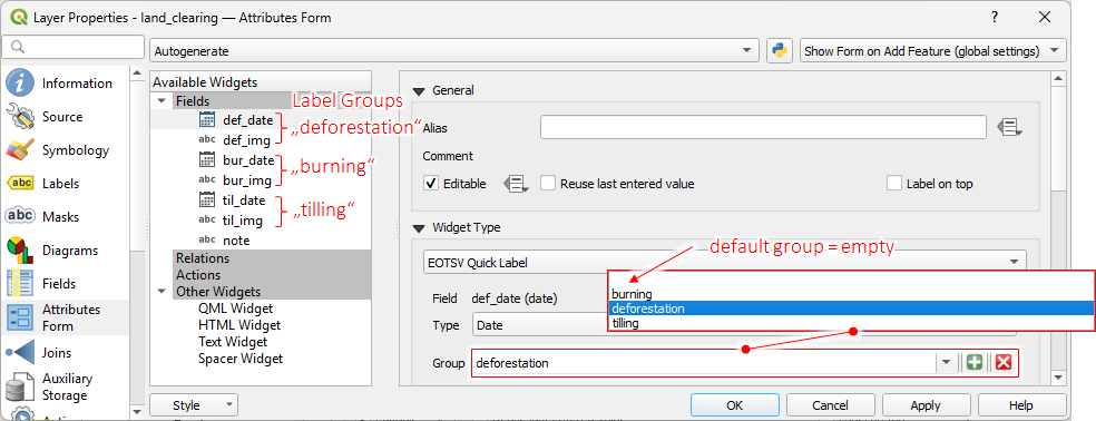
Fig. 8.3.1 Assigning quick label short cuts to label groups.

Apply the changes and close the layer properties. Now the map context menu allows you to trigger label shortcuts for each group separately.

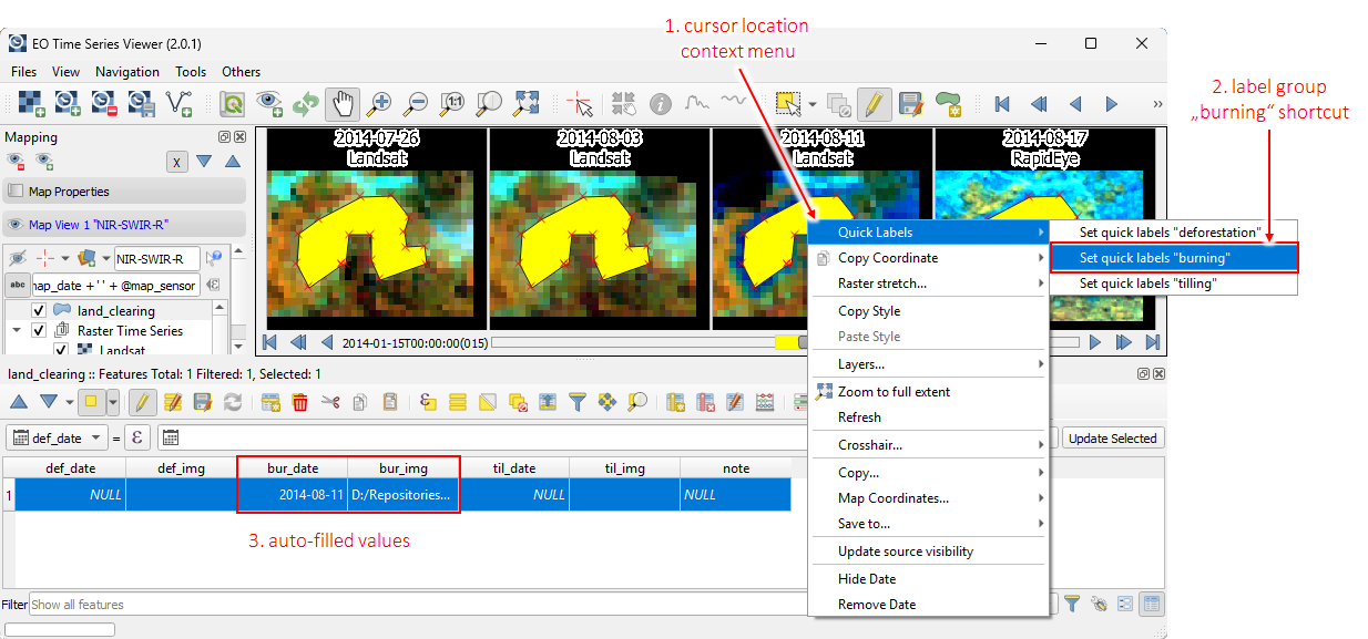
Fig. 8.3.2 Quick labeling using group-wise shortcuts