5. Map Visualization

The EO Time Series Viewer visualizes a temporal subset of a raster time series using a predefined number of map canvases. Each map belongs to an observation date and a Map View. Using multiple map views allows visualizing different band combinations at the same time.

../_images/mapview_concept.png — Fig. 5.1 Visualization of raster time series in different band combinations.

5.1. Map Properties

The map properties box is used to specify the:

number of maps per map view in horizontal and vertical direction,
width and height of each map
coordinate reference system (CRS)
map background color
the style how overlaid text will be styled

Click Apply to apply changes that affect the map size, number of maps and layout. By default the keep ratio option is cbc checked, i.e. height will increase/decrease as width.

../_images/mapview_concept_2x6x2.png — Fig. 5.1.1 The two map views, using a 6x2 map layout per map view.

5.2. Map Canvas

Maps in the EO Time Series Viewer can be used similar as known from the QGIS map canvas. The toolbar is used allows to activate tools to:

pan
zoom in and out ,
set the zoom to the raster pixel scale ,
or the map extent to that of the entire time series .

The identify tool can be used with the options to:

extract information for single pixels and vector features,
to load pixel profiles into a spectral library, or
to load temporal profiles into the temporal profile view.

If a vector layer is selected in the map view layer tree, vector features can be edited, added or removed.

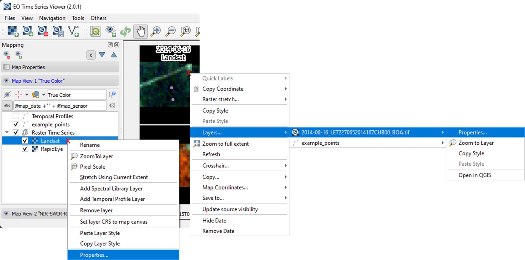
The context menu offers various shortcuts, e.g. to optimize the raster color stretch with respect to the current spatial extent, or to copy attributes related to map canvas and its observation date.

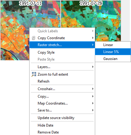
../_images/mapvis_map_context_menu.png — Fig. 5.2.1 The map context menu with shortcuts to optimize the color stretch

5.3. Map Views

A map view controls how the raster and vector data is visualized along the observation dates. Images linked to the same sensor are visualized with the same band combination and contrast settings. This means, optimizing the color stretch for a single raster layer will apply these settings to all other layers that belong to the same map view and sensor.

Each map view has its own layer tree, consisting of a raster layer for each sensor derived from them time series, as additional raster or vector layers.

You can add new Map Views using the button. This will create a new row of map canvases. Remove a map view with the button.
In case the Map View does not refresh correctly, you can ‘force’ the refresh using the button (which will also apply all the render settings).
Access the settings for individual Map Views by clicking in the mapview
You can use the button to highlight the current Map View selected in the dropdown menu (respective image chips will show red margin for a few seconds).

For every Map View you can alter the following settings:

Hide/Unhide the Map View via the button.
Activate/Deactivate Crosshair via the button. Press the arrow button next to it to enter the Crosshair specifications , where you can customize e.g. color, opacity, thickness, size and further options.
You may rename the Map View by altering the text in the Name field.

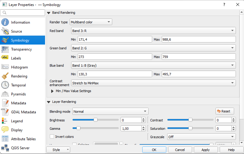
5.4. Layer Styling

Similar to QGIS, you can change the layer representation in the layer properties dialog. It can be opened from the layer tree or the map canvas context menu.

Fig. 5.4.1 The layer properties can be opened from either the layer tree (left) or a map canvas (right).

Fig. 5.4.2 The layer properties dialog.

5.5. Source Visibility

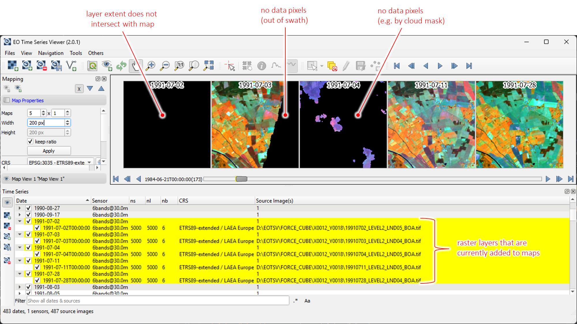
Earth observation time series often have gaps. For example, clouds may have been masked, the sensor did not cover the area that is currently visualized in the maps, or you just panned your maps outside the sensor swath.

In the time series panel, you can use the checkboxes cbu to hide the raster sources and observation dates which does not contain data for the given map extent.

Furthermore, the map context menu offers the Update visibility function. It checks for the entire time series, if the raster intersects with the map extent and contains valid pixel, i.e. pixel that are not set to any no-data value. Raster without valid pixels for the given extent will be unchecked, so that only maps and observation dates are shown for which valid raster pixel can be shown.

../_images/mapvis_update_visibility.gif — Fig. 5.5.1 The *Update visibility* function hides observations without valid pixels for the current map extent.

Note

To keep the time that needed to run the update visibility test for the entire time series short, it is carried out on 25 points, regularly sampled from the current map extent. Theoretically it’s possible, that none of the 25 points touches a valid pixel, while still the extent contains valid pixel inside the map extent. In that case the update visibility test might hide observations that still could provide useful information for a visual interpretation.

If in doubt, you can increase the number of points in the EO Time Series Viewer settings (Others > Settings) - of course at the expense of speed.

Furthermore, if the test runs too long, you can always cancel it in the task manager. Test results available until then are applied to the visibility of the sources.