6. Temporal Profiles

6.1. Loading

Temporal profiles can be loaded (a) interactively with the cursor location info tool, or (b) for point locations that are defined in a vector layer, using the read temporal profiles processing algorithms.

a) To load a single temporal profile on-the-fly, activate the identify cursor location value tool with option collect temporal profiles . Then click with the mouse on a map location of interest to extract the temporal profile for. If no other vector layer exists, the loaded profile will be added to a new created in-memory vector layer and visualized in the temporal profile view.

Fig. 6.1.1 Collecting temporal profiles.

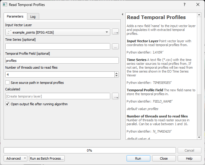
b) The read temporal profiles processing algorithm loads temporal profiles for multiple point locations. It can be started from menu bar Tools -> Read Temporal Profiles or the QGIS processing toolbox:

6.2. Data Structure

To visualize a time series in a plot window, the EO Time Series Viewer first extracts the multi-band and multi-sensor time series of the requested point locations. For a single point, the data related to a time series of length n is stored in a JSON struct that contains:

• a list date with n observation date items. Each date item is represented by an date-time string in ISO 8601 format,

• a list values with n value lists. Each value item is a list of raster band values in band order, i.e. the pixel profile that was observed at observation date_i at the point location,

• a list sensor with n sensor index values s, with 0 <= s < number of sensor_ids,

• a list with s >= 1 sensor_ids, one for each sensor the time series was observed by,

• a single sensor id is dictionary or its JSON string that contains the following key-value pairs:

  • nb (integer) number of bands

  • px_size_x (float) pixel resolution in x direction

  • px_size_y (float) pixel resolution in y direction

  • dt (integer) raster data type enumeration value, as taken from Qgis::DataType or GDALDataType

  • wl (optional) a list of nb float values with the band wavelengths

  • wlu (optional) a string value that describes the wavelength unit, e.g. nm or μm

  • name (optional) a sensor name, e.g. Landsat 8 or Sentinel-2

The following is a temporal profile JSON struct taken from the EO Time Series Viewer example data (Files > Add Example)

{"date":
    ["2014-01-15T00:00:00", "2014-03-20T00:00:00", "2014-04-21T00:00:00", "2014-04-29T00:00:00", "2014-05-07T00:00:00", "2014-05-15T00:00:00", "2014-05-23T00:00:00", "2014-05-31T00:00:00", "2014-06-08T00:00:00", "2014-06-16T00:00:00", "2014-06-24T00:00:00", "2014-06-25T00:00:00", "2014-07-02T00:00:00", "2014-07-10T00:00:00", "2014-07-26T00:00:00", "2014-08-03T00:00:00", "2014-08-11T00:00:00", "2014-08-17T00:00:00", "2014-08-19T00:00:00", "2014-08-20T00:00:00", "2014-08-26T00:00:00", "2014-08-27T00:00:00", "2014-09-12T00:00:00", "2014-09-20T00:00:00", "2014-09-28T00:00:00", "2014-10-06T00:00:00", "2014-10-14T00:00:00", "2014-11-07T00:00:00", "2014-11-15T00:00:00", "2014-12-17T00:00:00"],
 "sensor":
    [0, 0, 0, 1, 0, 1, 0, 1, 0, 1, 0, 2, 1, 0, 0, 1, 0, 2, 1, 2, 2, 0, 0, 1, 0, 1, 0, 1, 0, 0],
 "sensor_ids": [
    "{\"nb\": 6, \"px_size_x\": 30.0, \"px_size_y\": 30.0, \"dt\": 3, \"wl\": [0.49, 0.56, 0.66, 0.84, 1.65, 2.2], \"wlu\": \"micrometers\", \"name\": \"Landsat OLI\"}",
    "{\"nb\": 6, \"px_size_x\": 30.0, \"px_size_y\": 30.0, \"dt\": 3, \"wl\": [0.49, 0.56, 0.66, 0.84, 1.65, 2.2], \"wlu\": \"micrometers\", \"name\": \"Landsat ETM+\"}",
    "{\"nb\": 5, \"px_size_x\": 5.0, \"px_size_y\": 5.0, \"dt\": 2, \"wl\": null, \"wlu\": null, \"name\": null}"
    ],
"values": [
    [736.0, 1024.0, 1077.0, 4272.0, 2472.0, 1678.0],
    [769.0, 942.0, 763.0, 4345.0, 2138.0, 1043.0],
    [3894.0, 3993.0, 3916.0, 5516.0, 3799.0, 2876.0],
    [3307.0, 3440.0, 3436.0, 5822.0, 4161.0, 3220.0],
    [100.0, 210.0, 105.0, 1926.0, 798.0, 405.0],
    [640.0, 752.0, 595.0, 3822.0, 1725.0, 773.0],
    [3501.0, 3567.0, 3432.0, 4936.0, 3179.0, 2364.0],
    [242.0, 350.0, 216.0, 4046.0, 1606.0, 608.0],
    [146.0, 223.0, 122.0, 1907.0, 654.0, 244.0],
    [242.0, 361.0, 220.0, 3763.0, 1704.0, 615.0],
    [179.0, 356.0, 207.0, 3935.0, 1716.0, 617.0],
    [4573.0, 3682.0, 1944.0, 3504.0, 9692.0],
    [228.0, 415.0, 287.0, 3886.0, 1782.0, 677.0],
    [209.0, 405.0, 268.0, 3949.0, 1686.0, 668.0],
    [202.0, 400.0, 253.0, 3522.0, 1764.0, 715.0],
    [221.0, 412.0, 272.0, 3371.0, 1840.0, 724.0],
    [368.0, 534.0, 627.0, 1911.0, 1691.0, 1072.0],
    [7177.0, 5285.0, 4496.0, 4081.0, 4486.0],
    [669.0, 739.0, 768.0, 1795.0, 1921.0, 1457.0],
    [8686.0, 6353.0, 5231.0, 4679.0, 4948.0],
    [7187.0, 5676.0, 4295.0, 3733.0, 4332.0],
    [410.0, 567.0, 720.0, 1832.0, 2111.0, 1432.0],
    [328.0, 467.0, 562.0, 1613.0, 2195.0, 1596.0],
    [1667.0, 1640.0, 1632.0, 2849.0, 1854.0, 1444.0],
    [949.0, 1313.0, 1466.0, 2943.0, 3292.0, 2392.0],
    [1002.0, 1132.0, 1120.0, 2951.0, 2732.0, 1730.0],
    [288.0, 552.0, 626.0, 2189.0, 2440.0, 2198.0],
    [1448.0, 1662.0, 1688.0, 3874.0, 2997.0, 1932.0],
    [133.0, 229.0, 173.0, 1100.0, 645.0, 330.0],
    [387.0, 685.0, 662.0, 3231.0, 1775.0, 1088.0]
    ]
}

Note

Storing the entire temporal profile, including observations from all bands and different sensors, makes it possible to analyze different bands or spectral indices in parallel, without the need for a a new loading process.

The EO Time Series Viewer can store such JSON formatted temporal profile in any vector layer that supports string fields of unlimited length (most vector formats). Even better are formats that support JSON data types, like a GeoPackage. To use a vector layer field for temporal profiles requires to set its editor widget type to “Temporal Profile”.

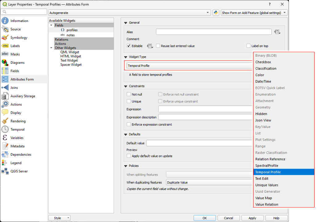
Fig. 6.2.1 Vector layer properties dialog with Attributes Form. The widget type of the “profiles” field is set to “Temporal Profiles”.

6.3. Visualization

Temporal profiles are visualized in the Temporal Profile View widget. If not already done, you can open it via Menu Bar -> View -> Temporal Profiles. The widget has a toolbar, a settings and a plot area (use the cursor to highlight them in the following image).

6.3.1. Toolbar

The toolbar allows to access the following actions:

Icon	Action
	Add temporal profile candidates permanently to the vector layer
	Create a new profile view
	Remove selected profile views
	Reload / refresh the plot
	Show only profiles whose vector layer feature are selected, for example in the map visualization or the an attribute table.
	Save changes to the vector layer
	Pan the map visualization to the coordinates of selected temporal profiles
	Zoom the map visualization to the coordinates of selected temporal profiles
	Deselect selected temporal profiles
	Open the attribute table to show the vector layer features for temporal profile layer selected in the settings table

6.3.2. Settings

The settings panel controls which and how temporal profiles are visualized. It allows to define one or more profile views

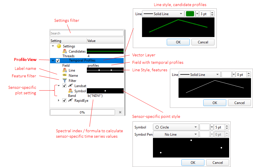
Fig. 6.3.1 The settings panel with one profile view to visualize the temporal profiles that are store in the attribute field profiles of the vector layer “Temporal Profiles”. The temporal profiles contain Landsat and RapidEye observations, whose visualization is handled separately.

A profile view defines:

• the vector layer and the vector layer field that contain the temporal profile data

• the line-style that is used to plot the profiles

• (optionally) a name that is given to the plotted profiles.

• (optionally) a filter to plot only profile that match with specific vector layer attributes

• for each sensor the profiles have observations from:

  • a point symbol, e.g. differentiate observations made by different satellites

  • a python expression to select the required band values or calculate a spectral index to be plotted.

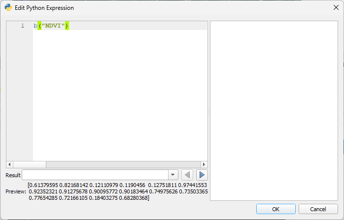
Fig. 6.3.2 The python expression dialog to define the formula that calculate sensor specific band values or spectral indices

In the sensor-specific python expressions the b(...) function is used to extract the band values as numpy array. These arrays can be used to define the formula to calculate the final plot values. If band wavelength and wavelength units are defined for the sensor, the b(...) function can be used with string inputs, like a band identifier or a spectral index acronym.

Example	Description
b(1)	return the values of the 1st band
b(1) * 100	return the values of the 1st band, scaled by factor 100
b('N')	returns the value of the near-infrared band (see settings)
(b(4) - b(3))/(b(4) + b(3))	returns the NDVI values for Landsat 8 legacy bands
(b('N') - b('R'))/(b('N') + b('R'))	returns the NDVI values, requires that wavelength information is provided for the sensor
b('NDVI')	returns the NDVI values, requires that wavelength information is provided for the sensor

The band identifiers and spectral index definitions are taken from the Awesome Spectral Index project You can inspect them in the EO Time Series Viewer settings (Others > Settings): For checked indices in the settings list, the profile view context menu will show a shortcut to set it in the python expression field.

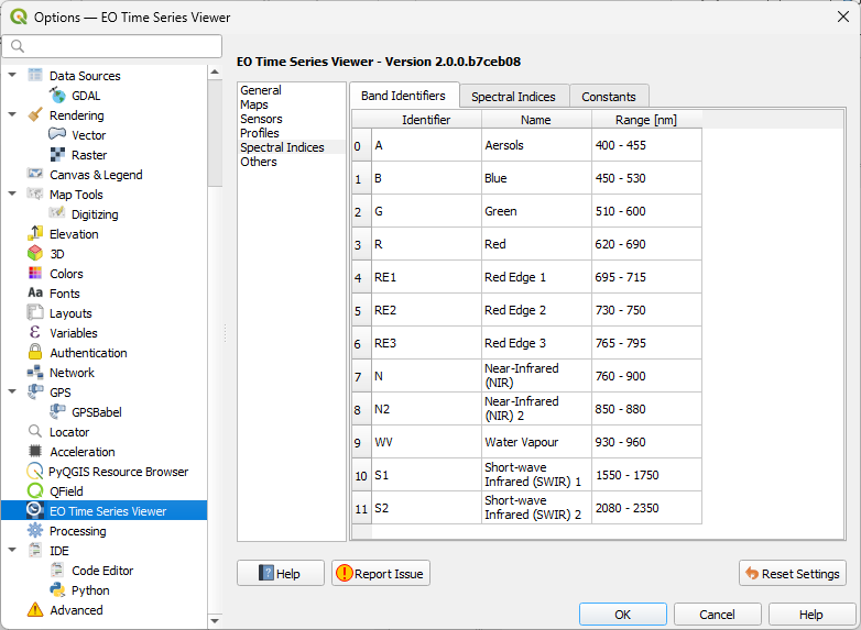
Fig. 6.3.3 EO Time Series Viewer Settings for spectral indices, list of band identifiers.

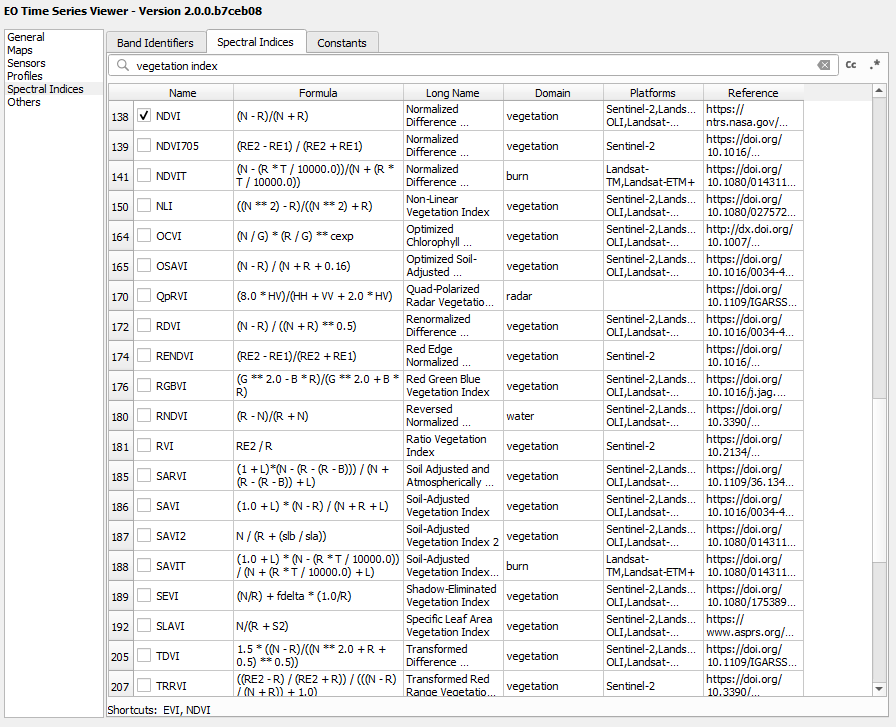
Fig. 6.3.4 EO Time Series Viewer Settings for spectral indices, spectral index definitions. Because NDVI and EVI are checked, they do appear as shortcuts in the context menu of the profile view (shown next figure).

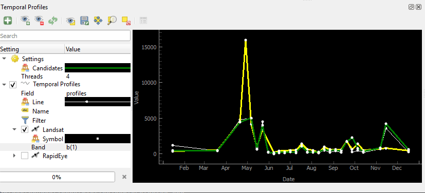
Fig. 6.3.5 The profile view context menu allows to active spectral indices fast.

6.3.3. Profile Plot

The profile plot panel visualizes the profiles as defined in the settings panel. The range of the x and y axis can be freely adjusted. To restore the default axis values, move the cursor to the the lower-left corner of the plot and click the click the [A] symbol.

A left-mouse click on a profile selects the corresponding vector feature, which becomes visible in an attribute table or map canvases that show the layer. Vice versa, a change of the selected points in a map canvas or rows in an attribute table does change which profiles are highlighted in the profile plot.

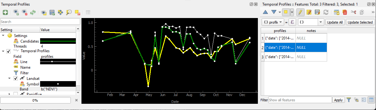
Fig. 6.3.6 Keep the right mouse button pressed to change the axis ranges. A selection of the lines also changes the selection of features in the attribute table and vice versa.

The context menu allows to enable or disable the display of a crosshair, data point information, and the time window that is visualized by maps in the Map Visualization. This time window can be adjusted interactively, e.g. to display the maps corresponding to an interesting event or sections in a temporal profile.

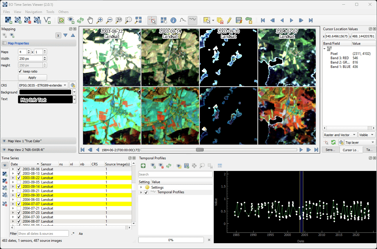
Fig. 6.3.7 Temporal profile plot with interactively changeable time window from which observations are displayed in the maps.