3. Graphical User Interface

3.1. Overview

This is how the EO Time Series Viewer’s interface looks after opening the example data (Files > Add Example).

You can use the mouse cursor to highlight different GUI parts and jump to its linked descriptions.

Note

Just like in QGIS, many parts of the GUI are adjustable panels. You can arrange them as tabbed, stacked or separate windows.

You can activate/deactivate panels under View ‣ Panels

3.2. Menu Bar

The menu bar give access to methods for handling data and visualization settings.

Fig. 3.2.1 Screencast of the menu bar

The Files menu allows to add new raster sources to the time series, and other raster and vector sources to overlay the time series data displayed in the map views. You can also start specialized import dialogs, e.g. to load raster data created with the FORCE processing framework.

The View menu can be used to show or hide the different panels and to add a new map view to the map widget.

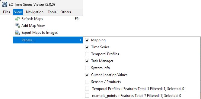
Fig. 3.2.2 The View menu allows to show or hide different panels.

The Navigation menu allows to select map tools for navigation to different spatial extents. It can also be used to copy the spatial extent from or to the map canvas of the main QGIS gui.

The Tools menu allows to start processing algorithms, e.g. to create a new temporal profile layer.

3.3. Tool Bar

In the tool bar you find tools to add and modify data and to adjust the data visualization.

Table 3.3.1 Toolbar buttons and what they trigger

Button	Function
	Add raster source to time series
	Add Time Series from CSV
	Remove all images from Time Series
	Save Time Series as CSV file
	Add vector data file
	Synchronize with QGIS map canvas
	Add maps that show a specified band selection
	Refresh maps
	Pan map
	Zoom into map
	Zoom out
	Zoom to pixel scale
	Zoom to maximum extent of time series
	Identify Pixels and Features
	Center map on clicked locations
	Identify cursor location values
	Identify raster profiles to be shown in a Spectral Library
	Identify pixel time series for specific coordinate
	Select Features
	Start Editing Mode
	Save Edits
	Draw a new Feature

Note

Only after ^{Identify Pixels and Features} is activated you can select the other identify tools (, , ). You can activate them all at once as well as of them, in case of the latter variant clicking in the map has no direct effect (other than moving the crosshair, when activated)

3.4. Map Visualization

The Map Views widget contains map canvases to visualize the observations of the raster time series. The slider on the bottom allows to change the temporal window of observation dates that is shown.

Each canvas relates to a Map View, in which all raster images of the same sensor are visualized with the same band combination and color stretch. Using multiple map views allows to visualize different band combinations of the same raster observation in parallel.

The Mapping panel allows to add or remove map views, change the canvas size and how canvases are displayed within a map view.

A detailed overview on the map visualization options is described in here

Fig. 3.4.1 Screencast of map visualization

3.5. Sensors / Products Panel

This panel show details on the sensors or image product types the time series consists of, e.g. the number of bands and the spatial resolution.

For better handling, the sensor names can be changed.

Fig. 3.5.1 The sensor panel show sensor details and allows to change their names

• name is automatically generated from the resolution and number of bands (e.g. 6bands@30.m). This field is adjustable, i.e. you can change the name by double-clicking into the field. The here defined name will be also displayed in the Map View and the Time Series table.

• n images: number of images within the time series attributed to the according sensor

• wl: comma separated string of the (center) wavelength of every band and [unit]

• id: string identifying number of bands, geometric resolution and wavelengths (primary for internal use)

3.6. Cursor Location Panel

This panel lets you inspect the values of a layer or multiple layers at the location where you click in the map view. To load these layer details, activate the identify cursor location value tool with option and use the mouse to click on the location of interest.

• The Cursor Location Value panel should open automatically and list the information for a selected location. The layers will be listed in the order they appear in the Map View. In case you do not see the panel, you can open it via View ‣ Panels ‣ Cursor Location Values.

  

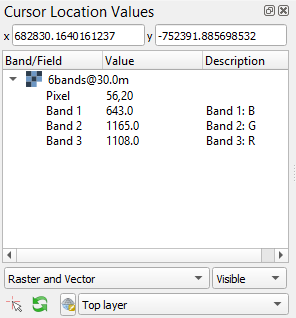
  Fig. 3.6.1 The cursor location value panel

• By default, raster layer information will only be shown for the bands which are mapped to RGB. If you want to view all bands, change the Visible setting to All (right dropdown menu). Also, the first information is always the pixel coordinate (column, row).

• You can select whether location information should be gathered for All layers or only the Top layer. You can further define whether you want to consider Raster and Vector layers, or Vector only and Raster only, respectively.

• Coordinates of the selected location are shown in the x and y fields. You may change the coordinate system of the displayed coordinates via the ^{Select CRS} button (e.g. for switching to lat/long coordinates).

Fig. 3.6.2 Screencast showing how to use cursor location info tool to show pixel and vector object values

3.7. Task Manager Panel

The Task Manager panel shows the progress of QGIS tasks which have been started from the EO Time Series Viewer. For example, to set the visibility of the individual raster sources, whether the source even contains valid raster pixels for the current displayed spatial map extent.

Fig. 3.7.1 The progress of the “update visibility” task is shown in the task manager panel (right).

3.8. Time Series Panel

The Time Series Panel show all raster sources that have been loaded into the time series. Each source can be enabled to disabled, so that is will be not be shown in the map views. Sources with a yellow background are currently displayed in a map canvas. The panel can be used to add additional sources, save the current sources into a CSV file, or remove sources from the time series.

Fig. 3.8.1 Showing and hiding of single observations sources in the time series panel.

3.9. Temporal Profile View

Here you can visualize temporal profiles that have been loaded for point coordinates.

To load a temporal profile, activate the identify cursor location value tool with option collect tempral profiles and click with the mouse on a location of interest.

The temporal profile view allows profiles from different vector layers to be shown together. A detailed description can be found in the Temporal Profiles section.

Fig. 3.9.1 Collecting temporal profiles.

3.10. Spectral Profile View

This panel is used to visualize the spectral profiles. To load a spectral profile from a raster image, activate the identify cursor location value tool with option collect spectral profiles and click with the mouse on a location of interest.

The spectral profile view panel is the same as used in the EnMAP-Box. For details, please visit the EnMAP-Box documentation for using spectral libraries.

Fig. 3.10.1 Collecting spectral profiles

3.11. Attribute Table

The attribute table can be used to show and edit vector layer attributes. In addition to many tools that are already known from the QGIS attribute table, the EO Time Series Viewer adds some shortcuts for a faster navigation and quick labeling.

• use the or button to select the next or previous feature

• activate the option to automatically pan the maps to selected feature(s)

• activate the option to automatically update the source visibility of the new map extent

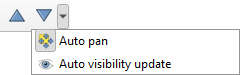
Fig. 3.11.1 Shortcut buttons to select the next or previous feature and options to updates the map visualization.

Fig. 3.11.2 Attribute panel and map visualization can be linked for panning the map extent automatically to selected vector features.